Escape time, and where the colours come from

The definition of the set says "the sequence stays bounded forever" — but no computer can wait forever. What it can do is exploit the theorem from the Mandelbrot chapter: once $z$ wanders further than 2 units from the origin, escape is guaranteed. So the infinite question becomes a finite loop:

z = 0
for n in 0 .. maxIterations:
    if |z|² > bailout:        # crossed the escape circle — verdict reached
        return n              # the escape time
    z = z² + c
return INSIDE                 # budget exhausted — presumed in the set

Two knobs matter. The iteration budget (maxIterations) decides how patient the renderer is: points hugging the boundary may survive thousands of steps before escaping, so deeper zooms need bigger budgets — Mandala raises it automatically with depth. The bailout is the escape test; any radius $\ge 2$ gives the same verdict, a freedom the smoothing below will spend.

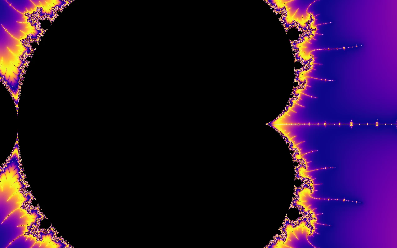
That step count $n$ is the escape time, and it is the raw material of every colour you see. Points far from the set escape in a handful of steps; points near the boundary survive far longer. Mapping the count through a palette turns the invisible boundary into weather — pressure lines crowding around the coast.

A period-3 island on the needle. Escape contours crowd the western antenna around a mini-copy: each shade is one more iteration survived before the orbit blew past the bailout circle. c ≈ −1.7548776662 · span 0.03 · open this view in Mandala →

From bands to gradients

Colouring by the raw integer count produces hard stair-steps: every pixel in a band took exactly the same number of steps. The fix is to notice how far past the escape circle the orbit landed on its final step, which pins down a fractional step count.

Here is where it comes from. Far outside the set, the $+\,c$ barely matters: $z_{n+1} = z_n^2 + c \approx z_n^2$, so each step roughly squares the orbit's size — $\log |z|$ doubles every iteration, which means

$$\log_2 \log |z_{n+1}| \;\approx\; \log_2 \log |z_n| + 1.$$

The quantity $\log_2 \log |z_n|$ is a clock that ticks forward by exactly $1$ per iteration once the orbit is escaping. Reading that clock at the moment of escape and subtracting it from $n$ cancels the arbitrariness of where the bailout circle happened to sit, leaving a smooth real number:

$$\nu \;=\; n + 1 - \log_2 \log |z_n|.$$

This smooth (continuous) escape count varies gradually between neighbouring pixels, so the bands melt into gradients.

One practical detail follows directly from the derivation: the approximation $z^2 + c \approx z^2$ is better the bigger $|z|$ is. So Mandala lets orbits run out to a circle of radius 256 ($|z|^2 > 65536$) rather than 2 — mathematically the verdict is identical, but the smoothing formula becomes far more accurate, which is why the gradients stay clean even under extreme magnification.

The cardioid cusp. Smooth (continuous) colouring: the fractional escape count blends the bands into gradients instead of hard stripes. c = 0.25 · span 0.15 · open this view in Mandala →

Palettes are a lens, not the truth

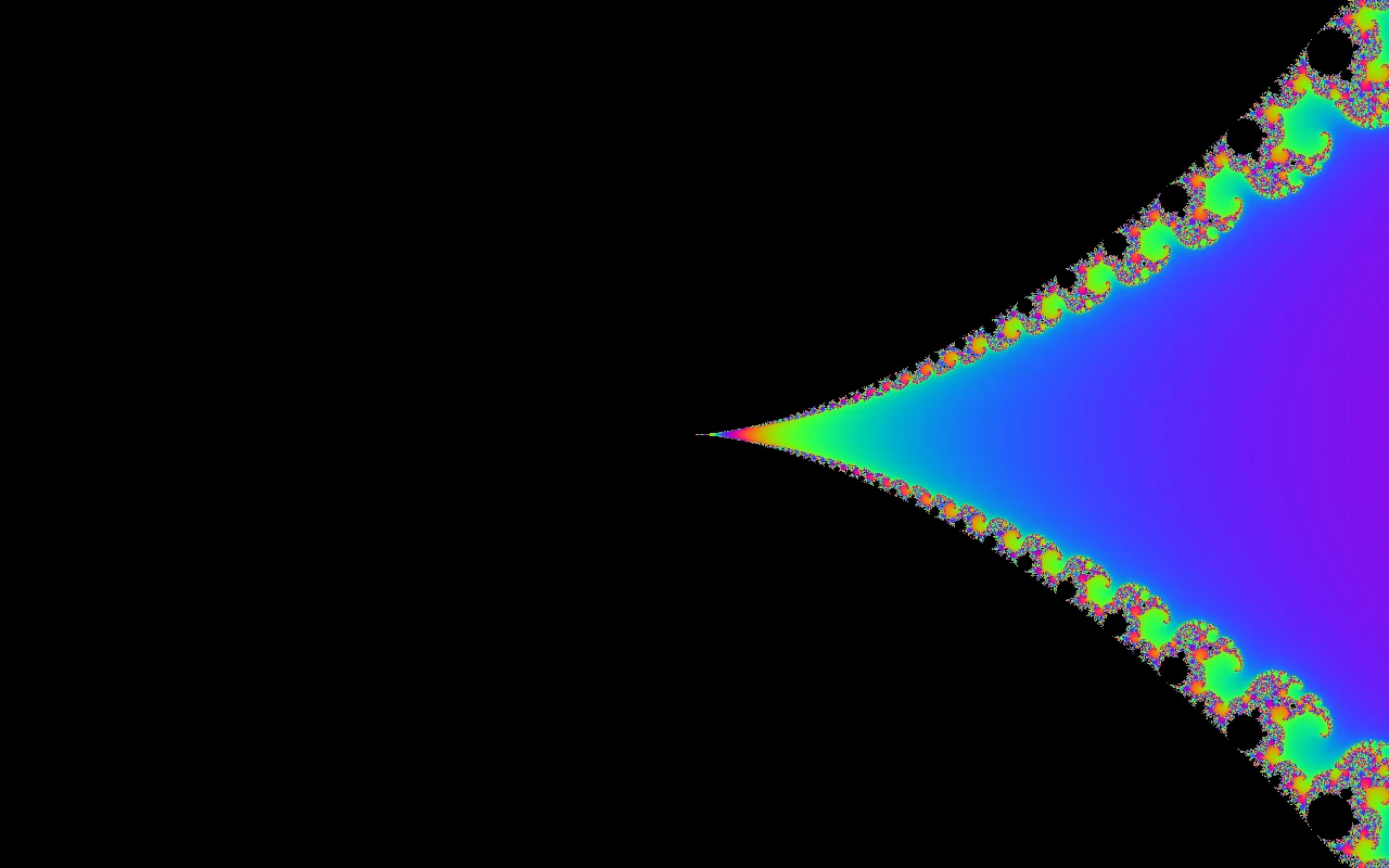
The escape count is the honest measurement; a palette is just how it's dressed. The pipeline is: smooth count $\nu$ → scaled by a colour-density setting → wrapped into a repeating phase → looked up in a palette. Because the palettes repeat cyclically, ever-larger counts keep cycling through colour rather than saturating — essential at depth, where counts run into the hundreds of thousands.

Mandala ships twenty-one palettes (plus a gradient editor to roll your own) — the same coordinates in a different palette can read as a different place, worth trying whenever a view feels flat. There's also a flow toggle that slides the palette phase continuously, which makes the contour structure around the set easy to see with your own eyes: what animates is the dressing, never the measurement. How all of that actually works — the phase-and-density pipeline, cosine palettes versus perceptual maps, the custom-gradient lookup table, and the classic histogram algorithm this renderer deliberately skips — is the next chapter.