What a fractal is

Most of the shapes mathematics is famous for are smooth. Zoom in on a circle and it flattens: magnify any little arc enough and it becomes indistinguishable from a straight line. Zoom in on a parabola, a sphere, an ellipse — same story. Smoothness means that detail runs out; under enough magnification, everything classical looks locally flat and boring.

A fractal is a shape where the detail never runs out. Magnify a stretch of it and you don't find a straight line — you find more structure, roughly as intricate as what you started with, and inside that structure more still, at every scale, forever. Benoît Mandelbrot coined the word in 1975, from the Latin fractus — broken, fragmented — because these are the shapes of broken things: coastlines, mountain ridges, river networks, clouds, lightning, the branching of lungs and trees.

The coastline paradox

The founding puzzle of the subject sounds like a trick question: how long is the coastline of Britain? Measure it with a 100 km ruler and you get one answer. Measure with a 10 km ruler and you get a noticeably bigger answer — the shorter ruler follows bays and headlands the long one stepped over. A 1 km ruler gives a bigger answer still, now tracing individual coves. The measured length doesn't converge to a true value as the ruler shrinks; it just keeps growing. A coastline behaves as if it were something more than a one-dimensional curve — as if length were simply the wrong kind of measurement for it.

Fractal dimension — measuring roughness

That "something more" can be made into a number. Cover the shape with boxes of side $\varepsilon$ and count how many boxes $N(\varepsilon)$ it touches. For a straight line, halving the box size doubles the count: $N \sim 1/\varepsilon$. For a filled square, halving the box size quadruples it: $N \sim 1/\varepsilon^2$. The exponent is the dimension — so take it as the definition:

$$N(\varepsilon) \sim \varepsilon^{-D}, \qquad D = \lim_{\varepsilon \to 0} \frac{\log N(\varepsilon)}{\log (1/\varepsilon)}.$$

For classical shapes $D$ comes out a whole number, and the definition agrees with intuition. The surprise is that nothing forces $D$ to be whole.

Take the Koch curve: start with a line segment; replace its middle third with the other two sides of an equilateral triangle; repeat on each of the four resulting segments, forever. Every construction step turns each segment into $4$ copies at $\tfrac13$ scale. So shrinking the measuring box by $3$ multiplies the count by $4$, and

$$D = \frac{\log 4}{\log 3} \approx 1.262.$$

Not $1$, not $2$: the Koch curve is genuinely between a line and an area — too crinkled to have a finite length (each step multiplies length by $\tfrac43$), too thin to enclose any. That in-between exponent is what "fractal dimension" means, and real coastlines measure out the same way, typically around $D \approx 1.2$–$1.3$.

Three kinds of self-similarity

Fractals repeat themselves across scales, but in three distinct ways:

Exact self-similarity — constructed fractals like the Koch curve or the Sierpiński triangle contain perfect copies of themselves, by construction: the recipe is literally "replace each part with scaled copies of the whole".

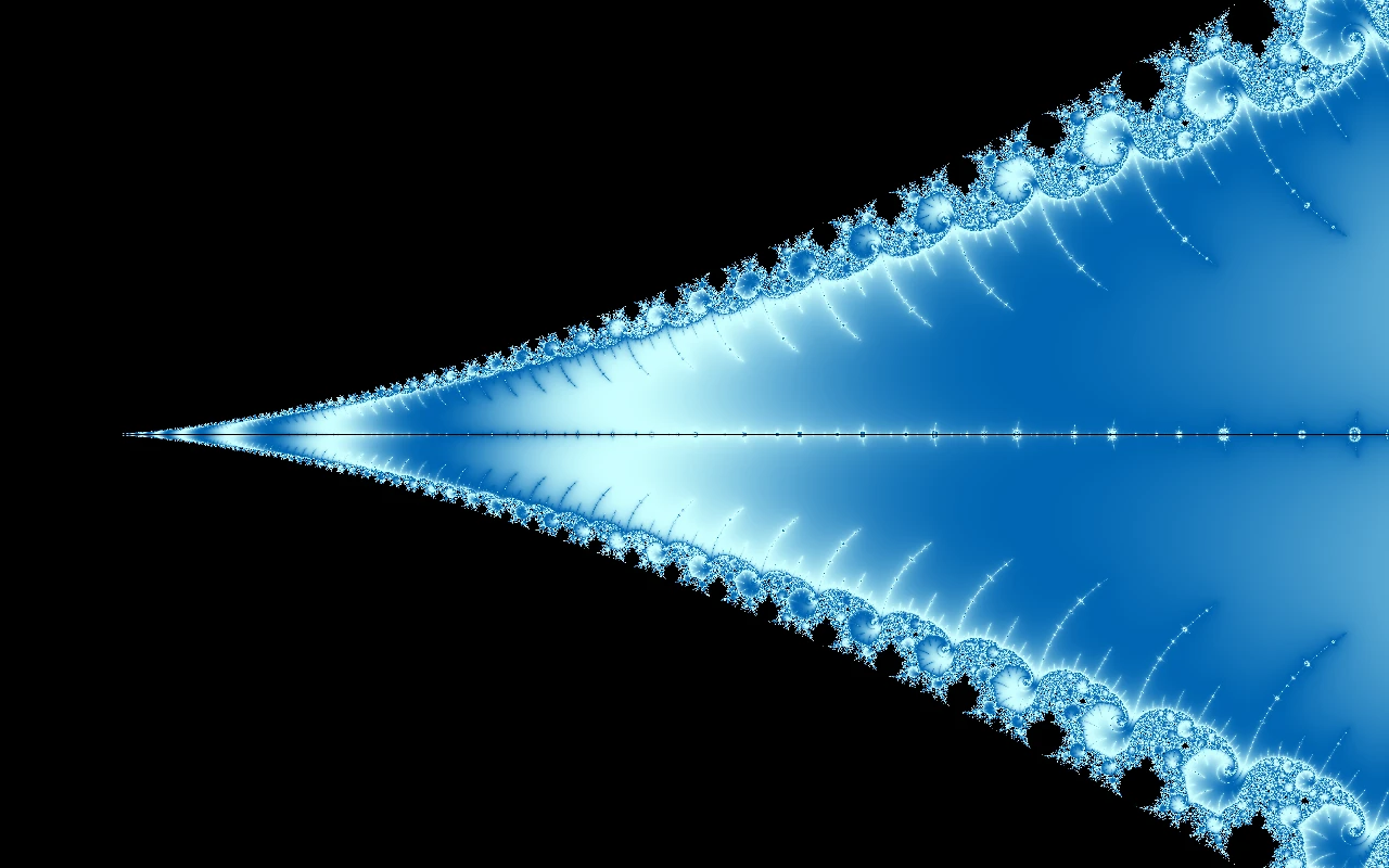
Quasi-self-similarity — the Mandelbrot set's kind. The boundary carries copies of the whole set — the minibrots — provably infinitely many of them: renormalization (Douady–Hubbard) shows small copies are dense along the boundary, so magnifying any boundary stretch far enough reveals one. But no two are identical: each sits in its own web of filaments, squeezed and decorated differently. The set echoes itself without ever repeating itself, which is why exploring it stays interesting in a way that zooming a Koch curve does not.

Mini-Mandelbrot. A complete copy of the whole set, seven ten-thousandths of a unit wide, on the western antenna. c ≈ −1.7497 · span 7×10⁻⁴ · open this view in Mandala →

Statistical self-similarity — nature's kind. No piece of a coastline is a copy of another, but the statistics of the roughness (how wiggliness scales with ruler size) are the same at every scale. This is the sense in which clouds, terrain and river networks are fractal.

Where escape-time fractals fit

The fractals in this explorer are not built by a cut-and-replace recipe. They emerge. Take one rule — $z \mapsto z^2 + c$ — iterate it, and ask which points stay bounded (the Mandelbrot chapter makes this precise). The interior of the answer is tame; all the fractal behaviour concentrates on the boundary, the knife-edge between staying and escaping.

And that boundary is about as extreme as the definition above allows: its fractal dimension is exactly $2$ — the maximum possible for a curve in the plane — a deep theorem of Mitsuhiro Shishikura (Annals of Mathematics, 1998). A one-line rule, iterated, produces a curve so crumpled that by the box-counting yardstick it is indistinguishable from an area. Dimension $2$ does not by itself decide whether the boundary actually has positive area, though — that is a separate and still-unsolved question. That is the shape this field guide is about, and the next chapter defines it properly.